Making sense of a mess with the kaleidoscope transform

One of my daughter’s aunts submitted the first photo for a Springbok Puzzle contest and Springbok has chosen to display it on their Facebook fan page. See the firs picture below.

The second picture is with my favorite tiling transformation applied to the first one. (Made with the image functions of Mathematica.) In mine opinion the transformed image emphasizes the qualities of the first image since it brings some order and sense to the mess.

Caterpillar writing of the kanji “butterfly”

A resent discussion over the quote

Just when the caterpillar thought the world was over, it turned into a butterfly.

reminded me of a haiku by Bashō

胡蝶にもならで秋経る菜虫哉
kochoo ni mo narade aki furu namushi kana

The translation to English I like the most is

Deep into autumn
and this caterpillar
still not a butterfly

Remembering this haiku gave me the idea to write the kanji for “butterfly” with the caterpillar pen within the iPad app Sumo Paint.

I even wrote — or more precisely drew — the original haiku in Japanese using the iPad app Zen Brush. (Well the result is not that great, but still I wanted to share the idea …)

Below are some variations of the above images. First, thicker caterpillars:

Second, a Percolator-ed version of the haiku writing with Zen Brush:

Markov Chains and N-Grams in Mathematica

While reading the book “Programming in Lua” I reached the chapter where it is described an implementation of a random text generation algorithm using Markov chains and N-grams. I implemented a similar algorithm 10 years ago. My first encounter with this algorithm was when I was a teenager — I read a description of it in Martin Gardner‘s column in the Russian translation of “Scientific American.”
Instead of digging out that old implementation, I decided to write a new one from scratch in Mathematica and that turned out to be surprisingly easy.
The easiness came from the available implementations of multi-dimensional sparse arrays (SparseArray) and weighted random sampling (RandomSample). The code I wrote can be run with N-grams of any N; the implementation in the book “Programming in Lua” 2nd ed. is for 2-grams — see Chapter 10.2 of the book.

Below are given screenshots of texts generated by the algorithm using Darwin’s “The Origin of Species.” (Also readily available within Mathematica.) From them you can see that the 5-gram generated text makes more sense than the 2-gram one. All 4 randomly generated texts start from the same place in the book.

Here is the Mathematica code:

(* The argument numberOfPreviousWords is for the size of the N-grams. *)
(* The argument numberOfWords is for the size of the randomly generated text. *)
Clear[MakeRandomText]
Options[MakeRandomText] = {"StartNGram" -> Automatic};
MakeRandomText[text_String, numberOfPreviousWords_Integer, 
   numberOfWords_Integer, opts : OptionsPattern[]] :=
  Module[{textWords, words, PickWord, wordToIndexRules, 
     indexToWordRules, ntuples, markovMat, inds, randomTextWords, 
     startNGram, startNGramOpt = OptionValue["StartNGram"]},
    textWords = StringSplit[text];
    words = Union[textWords];
    wordToIndexRules = Dispatch[Thread[words -> Range[Length[words]]]];
    indexToWordRules = Dispatch[Thread[Range[Length[words]] -> words]];
    PickWord[inds_] := 
     RandomSample[Normal[markovMat[[Sequence @@ inds]]] -> words, 1][[1]];
    PickWord[ss : {_String ..}] := PickWord[ss /. wordToIndexRules];
    ntuples = Partition[textWords, numberOfPreviousWords + 1, 1]; 
    markovMat = 
     SparseArray[{}, 
      Table[Length[words], {numberOfPreviousWords + 1}]];
    Do[
     inds = Apply[Sequence, t /. wordToIndexRules];
     markovMat[[inds]] = markovMat[[inds]] + 1,
     {t, ntuples}];
    startNGram = 
     If[NumberQ[startNGramOpt] && startNGramOpt <= Length[ntuples], 
      ntuples[[startNGramOpt]], RandomSample[ntuples, 1][[1]]];
    randomTextWords = 
     Nest[Append[#, PickWord[Take[#, -numberOfPreviousWords]]] &, 
      Most@startNGram, numberOfWords];
    StringJoin @@ Riffle[randomTextWords, " "]
    ] /; 2 <= numberOfPreviousWords <= 5;

My first entry for the One-liner competition at WTC 2012

My first entry for the one-liner competition at the Wolfram Technology Conference 2012 makes wallpaper autostereograms. (See http://en.wikipedia.org/wiki/Autostereogram.)
Using the correct pupil focus you should see six black balls in front of a black wall, six red balls in front of a black wall with circular holes, and a red wall with circular holes in front of five black balls/disks. When you enter the gallery if you focus correctly on one of the images you will see the rest without refocusing.

You can also try to focus on the slide show. (I can focus easily on the slideshow, but this might be because I know what I am going to see and because of my high resolution screen…) Because the slideshow images are smaller the number of perceived balls / disks increases with 1. For example, apparent seven balls are seen on the first image.

This slideshow requires JavaScript.

 

Evaluating several times this code would produce the images with the red balls and the red wall:
{u, v}=Point/@GatherBy[RandomReal[1,{8000,2}],Norm[#-.5]<.33&];
F[p_,s_]:=Translate[p,{#,0}]&/@Range[0,4,s];
Graphics[{F[u,1],Red,F[v,.8]},ImageSize->1200]

My third entry for the One-liner competition at WTC 2012

Here is a screenshot of my third entry for the one-liner competition at the Wolfram Technology Conference 2012. I took the TIGER shapefile data that gives the geometry edges of various geo-objects in the Champaign county, replaced the edges with polygons, and sharpened the result image.

That third entry did not get mentioned in any of the categories of the competition (“dishonorable mention” , “honorable mention” , “winners” ).

Won the second place in the One-liner competition at the Wolfram Technology Conference 2012

I was a speaker at the Wolfram Technology Conference 2012. I presented two talks and I also submitted three entries for the One-liner contest. The contest is to write Mathematica code 140 characters long or less that would impress the judges. I won the second place with one of my submissions called “Translating Chinese characters into a folk-like melody”, which should have been named “Translating Chinese characters into a Bulgarian folk-like melody”, but I didn’t want to hint to the judges who is the contestant. (There were only two Bulgarians at the conference.)

Here are the two character sequences I used

“䥰仨䯈䵘䵘䥰䯈勐仨仨䯈䥰塈嚸唨仨䵘䯈䥰䥰仨䯈䵘䵘䥰勐仨勐仨仨䯈䥰塈嚸塈唨仨䯈䵘䀐”
“䚌䙮䙮䙮䙮䚌䚌䙮䙮䙮䙮䚌䚌䙮䙮䙮䙮䚌䝀䚌䙮䙮䙮䙮䚌䙮䙮䙮䙮䙮䙮䚌䙮䙮䙮䙮䙮䙮䚌䛈”

in order to produce the main voice in the this composition of mine:

https://soundcloud.com/anton-gramsci/bulgarian-folk-melody

Further details follow. I transposed the original melody to start from E not from F because this made the note specification for SoundNote to be shorter. Not short enough, though. So that is why I did the remapping from strings to integers — SoundNote can take integers as note specifications. With this approach, though, I wasn’t able to specify pauses and chords. So I prolonged one of the notes in the middle of the melody and changed the power chord at the end to be a single note in a lower octave.

Moku Hanga Distortions

Here is another take on moku hanga distortions with the iPad app Percolator.

Arizona Teas Warholized

Because of my liking of tea, kanji, and moku hanga I came up with this collection of processed versions of the same photo. The collection is quite Warhol-esque, because of Andy Warhol’s inclination to make matrices of canned food and general propensity to put the same motif (possibly transformed) in series.

A slide show, though, presents better the image processing I did with the iPad apps Percolator and Moku Hanga HD.

This slideshow requires JavaScript.

Tiger Shark Data Analysis

Few weeks ago I was at a movie screening and panel discussion about tiger sharks at the Museum of Art of Fort Lauderdale. During the reception I talked to the main presenter — prof. Shivji — and some of his students about the shark data they have and boldly offered to do data mining on it. My angle was, “ok, let’s drop the usual statistics with its inductive jumps and use the more straightforward of approach data mining”. I asked what is the volume of the shark data, and it turned out only eleven shark are followed. This diminished my enthusiasm, but may be they had lots of data for each shark.

So I grabbed the data available at the web site “Track Your Tiger Shark”, and started doing plots, histograms, and harvesting of weather and elevation data for the sharks locations at the times they showed up. The location and time of the tagged sharks are recorded when their fins are above the water surface. (I.e. the tracking devices on their fins are above the surface.)

I worked mostly with the sets “Bermuda 2009” and “Bermuda 2010”. I used the Google elevation service to get the depth of the water at the shark locations, and Mathematica’s WeatherData interface for air temperature and wind direction and speed.

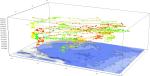
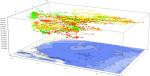
I would not say that the data matchings, various clusterings, and plots uncovered something new. Except one, all attempts for correlation and law discoveries were either hard to interpret (probably meaningless), or easy to explain. For example, in the 3D histogram of the shark locations we can see that the sharks would most likely spend their time in shallow waters around the islands where food is easier to find.

I also plotted histograms, “trajectories”, and polar plots of depth, speed, average time to show up, and few others. (See the gallery below)

The most interesting find from all this activity is illustrated in the plot below — the sharks prefer to swim against the wind. For each shark I calculated its assumed direction of swimming and compared it to the wind direction at that time and geographical point. The comparison is done by calculating the cosine of the angle between the wind and shark directions. (If the cosine is -1, the directions are opposite; if it is 1 the directions coincide.) When we make this comparison we need to also look at the wind velocities and the time intervals between two consecutive points of the sharks showing up. I made histograms of the intervals but did not make correlation study with the cosines. (Well, not yet.)

I assume at the surface the water has the same direction as the wind. I have two conjectures why sharks would prefer swimming against the wind.
1. Other (smaller) fish follows the water direction, and, hence, it is easier to catch.
2. It is easier to breathe.

To clarify the second point, let us note, that in order to breathe most shark species have to constantly swim forward or, if still, face a current in order the water to flow over their gills. Although I am not sure is the respiratory system of the tiger sharks like this, it seems that they might prefer facing the current especially if they are younger — note the plots of the juvenile sharks. (They have “juvenile” next to their names.) The sharks from the “Grand Cayman” data set disprove the conjecture — see the row before the last. The last row of plots should be ignored because for too many of the shark locations the wind data is missing.

In the gallery you would find images of a 3D shark location histogram, the space-time trajectory of one of the sharks, the space-time (3D) and space (2D) trajectories of all sharks, and a table of plots of sorted cosines of wind direction minus shark direction for each shark.

Rock Paper Scissors Lizard Spock

In one of the episodes of “The Big Bang Theory” was introduced a modification of the game “Rock, Paper, Scissors” called “Rock, Paper, Scissors, Lizard, Spock” — see “Rock Paper Scissors Lizard Spock” on Youtube .

Here is a graph illustrating the relationships of “Rock, Paper, Scissors, Lizard, Spock”:

The list of rules “Rock, Paper, Scissors, Lizard, Spock” is:

01. Scissors cuts Paper;
02. Paper covers Rock;
03. Rock crushes Lizard;
04. Lizard poisons Spock;
05. Spock smashes Scissors;
06. Scissors decapitates Lizard;
07. Lizard eats Paper;
08. Paper disproves Spock;
09. Spock vaporizes Rock;
10. Rock crushes Scissors.

Here is the Mathematica code for the graph:
GraphPlot[{{"Scissors" -> "Paper", "cuts"}, {"Paper" -> "Rock", "covers"}, {"Rock" -> "Lizard", "crushes"}, {"Lizard" -> "Spock", "poisons"}, {"Spock" -> "Scissors", "smashes"}, {"Scissors" -> "Lizard", "decapitates"}, {"Lizard" -> "Paper", "eats"}, {"Paper" -> "Spock", "disproves"}, {"Spock" -> "Rock", "vaporizes"}, {"Rock" -> "Scissors", "crushes"}},
EdgeLabeling -> True, VertexLabeling -> True, DirectedEdges -> True,
Method -> "CircularEmbedding"]


(It turns out this is already done:
[1] http://www.thinkgeek.com/tshirts-apparel/unisex/generic/b597/?srp=3 ;
[2] https://www.rockitrigs.com/pictures/ShirtChuckDefeatsAll1.jpg .)

And, just to be complete, here is a graph illustrating the relationships of “Rock, Paper, Scissors”: